Visual Odometry Implementation from Scratch
Introduction
This is the first-ever post of my blog; so I will give it a try. This post is about things that I went through when I tried to implement a simple monocular visual odometry from scratch. For a programming language, I choose MATLAB because it is easy-to-use and fast for prototyping a project.
Disclaimer: This is not a state-of-the-art implementation. This simply serves the purpose of learning.
The Problem
To give a general idea, visual odometry (VO) is an algorithm that aims to recover the path incrementally, by using the visual input from cameras, and hence the name. It can be considered as a sequential structure from motion, as opposed to hierarchical structure from motion. Imagine a robot or an agent, attached with a calibrated camera $C$, moves through an environment and receives the image continuously. The images $I_k, I_{k-1}$ are taken at different time steps $k$ and $k-1$, which corresponds to the camera pose $C_k$ and $C_{k-1}$ respectively. The task of VO is basically to retrieve the transformation matrix $T = \left[R \lvert t \right]$ that relates two camera poses, and concatenate all the transformaitons $T_k$ to get the current camera pose:
$$ C_{t} = T_{t,t-1}C_{t-1}$$
Getting Things Up & Running
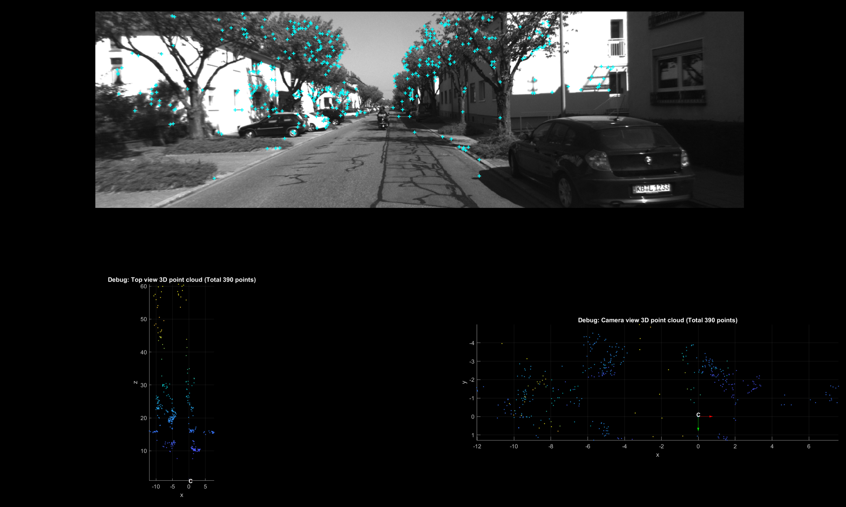
I first have an initialization function vo_initialize.m that takes two image frames, establishing keypoint correspondences between these two frames using KLT feature tracker, estimating relative camera pose, and finally triangulating an initial 3D point cloud landmarks. I admit that these may sound lacking of excitement (as they are something that is well understood in the computer vision community), but they are not easy to implement from scratch in a single sit.
Feature Detection
This is a simple plementation of Harris corner detector. For each pixel $(u,v)$, we calculate a score
$$R = det(A_{u,v}) - {\lambda}trace^2(A_{u,v})$$
where
$$ A_{u,v} = \begin{bmatrix} \sum{I^2_{x}} & \sum{I_{x}I_{y}}\ \sum{I_{x}I_{y}} & \sum{I^2_{y}} \end{bmatrix} $$
and $I_x, I_y$ are the image gradients in $x$ and $y$ direction respectively.
I_x = conv2(img, [-1 0 1; -2 0 2; -1 0 1], 'valid');
I_y = conv2(img, [-1 -2 -1; 0 0 0; 1 2 1], 'valid');
I_xx = double(I_x.^2);
I_yy = double(I_y.^2);
I_xy = double(I_x.*I_y);
I_xx_sum = conv2(I_xx, ones(patch_size), 'valid');
I_yy_sum = conv2(I_yy, ones(patch_size), 'valid');
I_xy_sum = conv2(I_xy, ones(patch_size), 'valid');

pad_size = floor((patch_size+1)/2);
scores = (I_xx_sum.*I_yy_sum - I_xy_sum.^2) - lambda*(I_xx_sum + I_yy_sum).^2;
scores(scores < 0) = 0;
scores = padarray(scores, [pad_size pad_size]);
After calculating the score, we simply select $k$ keypoints with highest scores (with non-maximum suppression).
scores_pad = padarray(scores, [r r]);
score_size = size(scores_pad);
keypoints = zeros(2, k);
for i = 1:k
    [~, idx] = max(scores_pad, [], 'all', 'linear');
    [row, col] = ind2sub(score_size, idx);
    keypoints(:, i) = [row; col] - r;
    scores_pad(row-r:row+r, col-r:col+r) = 0;
end
KLT Feature Tracker
…
Pose Estimation
…
Triangulation
…
The result of vo_initialize.m seems reasonable. Good to go!
Problems from Previous Implementation
…
Estimate World Camera Pose
…
Bundle Adjustment
Bundle adjustment is a very cool concept. To put it simply, it is an optimization algorithm used to refine the estimated trajectory.
In this implementation, a motion-only bundle adjustment is implemented, which optimizes only the camera orientation $R$ and position $t$. This implies that
Results
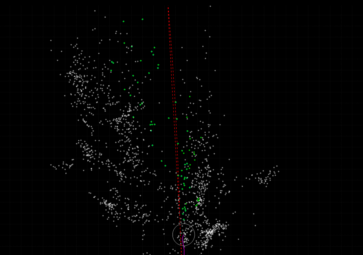
Putting it all together, the vo_initialize.m function initializes the VO pipeline, creating initial 3D point landmarks, extracting initial keypoints, and estimating the initial pose of the camera. The vo_process.m sequentially extracting and tracking image features from an image frame, across frames, and simultaneously estimating the pose of the camera. Bundle adjustment is also implemented to refine the estimated pose at each step. Lastly, new 3D points are regularly created as the number of currently tracked keypoints is shrinking over time. The following is the final result.
From the video, it is obvious that this is not a state-of-the-art implementation. There are various components that are not implemented. As we can see, the estimated trajectory starts to deviate from the ground truth after some time, due to the scale drift–a common problem in monocular VO. The estimated trajetory also wiggles slightly, probaly due to the fact that the full bundle adjustment is not implemented. And the most importantly, I did not try to implement a loop closure.
Reflections
The task of implementing VO from scratch may sound lacking of excitement. I believe that the conventional pipeline of VO and SLAM is something that is already well-understood in the computer vision community. What I realize is that academic papers usually have missing steps that are left for the readers to figure out. Here, I tried to connect those steps and the result stands as a self-assesment of my understanding.